Function Optimisation Using PyTorch

PyTorch is a python library for machine learning. This library includes tools for creating models and, importantly for this post, tools for training these models. Machine learning is really just fancy optimisation. So can we use these fantastic tools for machine learning to perform the (simpler) task of function optimisation? Can we use our fancy electric screwdriver to hammer a nail?

Optimisation

Optimisation is commonly used to solve multivariate equations iteratively, or to find the largest or smallest point of a function. Generically, optimisation is performed by minimisation of an objective function. The value of the objective function is not necessary what we care about, but is related to the value of interest.

That’s an abstract way of saying that the objective function transforms whatever optimisation problem we want to solve into a minisation problem.

Some examples:

Minimises the negative of the function thereby maximising the function.

Minimises the differences between \(a\) and \(f(\theta)\) and so the minimiser will find the parameters \(\theta\) which results in a function value of \(a\).

I have presented the above with a scalar function output, but similarly applies to vector functions.

Gradient Descent

One method of solving an optimisation problem is “gradient descent”. By calculating the gradient of the function with respect to the inputs, we can update the inputs to a value which will reduce the value of the objective function.

This is represented on the figure below.

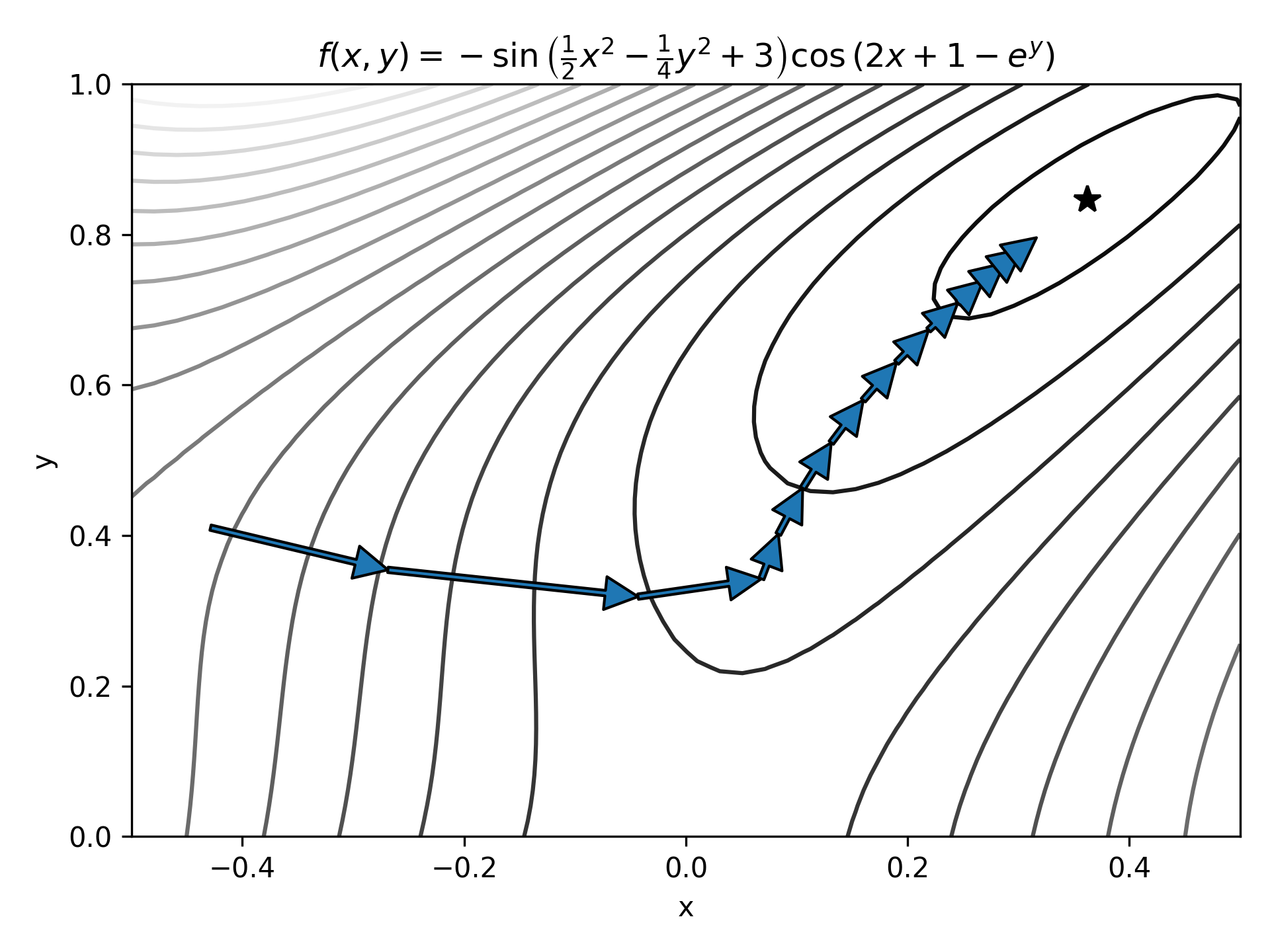
Starting from a point on the function space, the gradient is calculated and then the parameters (x, y position) are updated reducing the function value.

Calculating the gradient of a known function can be as simple as finding the gradient of the function. Although, if the function is known, then this offers more efficient methods of finding the minimum values. In the likely case where the function is unknown then how do we get the gradient? Enter PyTorch.

PyTorch

PyTorch is a python library used for machine learning. Machine learning is just complicated optimisation. PyTorch centres around an efficient automatic differentiation system which propagates gradients through calculations as they happen giving accurate estimations of gradients without any knowledge of the function required.

PyTorch as a Generic Function Optimiser

We can apply Pytorch to an optimisation problem quite easily:

import torch

def pytorch_fopt(f: callable, a: torch.Tensor, n_ev=1000, lr=1e-2) -> torch.Tensor:
    a.requires_grad = True
    for _ in range(n_ev):
        a.grad = torch.zeros_like(a)
        v = f(*a)
        v.backward()

        a.requires_grad = False
        a -= lr*a.grad
        a.requires_grad = True
    return a.detach()

The function above is quite short but some things in it appear a little cryptic. Let’s break it down.

First, we take the initial point, a, and we tell torch that we want to calculate the gradient with respect to it. a is a tensor and may not necessarily be a single scalar value, but can be a vector. In the example given above it would have been a pair of numbers - a 2D coordinate.

a.requires_grad = True

Then we start a loop - this is where we start stepping down the gradient of the function - and reset the gradient to a value of zero. If we don’t do this every loop, we will accumulate gradient erroneously as more calculations are performed.

for _ in range(n_ev):
    a.grad = torch.zeros_like(a)

Next we calculate the value of the function, and then we backpropagate the gradient through the calculation by calling backward.

v = f(*a)
v.backward()

Now we have the gradient with respect to the input a calculated for us - stored in a.grad. We want to update a to minimuse the function value, so we subtract the gradient multiplied by a learning rate. However, we don’t want this step to affect any gradients (PyTorch would complain) so we detach the autograd system temporarily.

a.requires_grad = False
a -= lr*a.grad
a.requires_grad = True

Repeating this process a few times gives us, hopefully, a good solution to our optimisation problem!

Let’s test it. For the function

What is the maximum point? Well, by inspection we know that it should be at \(x = y = \pi/2\) as that is when the \(\sin\) function is at its maximum.

Let’s find the value using our optimiser. If we want to find the maximum value, we find the minimum of the negative function:

def f(x: torch.Tensor, y: torch.Tensor) -> torch.Tensor:
    return -torch.sin(x)*torch.sin(y)

Then the solution can be found by running:

pytorch_fopt(f, torch.zeros(2))
# result: tensor([0., 0.])

Ah, that’s not what we wanted. What’s going on there then? It seems that at input of zero, and function value of zero, the gradient is also zero (makes sense). So let’s change our starting point a little:

Then the solution can be found by running:

pytorch_fopt(f, torch.zeros(2)+0.1)
# result: tensor([1.5705, 1.5705])

Ah that’s better! \(1.5705 \approx \pi/2\), the right answer. We used a very simple bit of code to optimise the function taking the gradient from PyTorch. What if we didn’t use a custom optimiser? PyTorch has a slew of their our - could we use them?

PyTorch Optimiser

PyTorch has a bunch of implemented optimisers available including Adam (ADAptive Moment estimation) and SGD (stochastic gradient descent). These are the two that I am most familiar with and the ones I’ll be using here. Stochastic gradient descent is similar to gradient descent, but it randomly walks ‘up’ the gradient to avoid getting stuck in local minima. Adam is similar, but includes a momentum parameter to further “steamroll” through small local minima which would otherwise trip up normal GD.

The optimiser is constructed by giving it the parameters it is to change, as well as passing in settings dictating how the optimiser will run.

import torch

a = torch.Tensor([1, 1])
opt = torch.optim.Adam([a], lr=0.1)

We can now adapt the pytorch_fopt function to use one of the pytorch optimisers:

def pytorch_fopt(f: callable, a: torch.Tensor, nfev=100, opt=torch.optim.Adam, **opt_kwargs):
    a.requires_grad = True
    opt = opt([a], **opt_kwargs)
    for _ in range(nfev):
        opt.zero_grad()
        v = f(*a)
        v.backward()
        opt.step()
    return a.detach()

We use it similarly to before:

pytorch_fopt(f, torch.zeros(2)+0.1, nfev=100, lr=0.1)
# result: tensor([1.5663, 1.5663])

Not quite as good as before, why might that be? For big, complex, problems Adam is the more efficient choice. For this very easy task Adam is struggling a little bit given the same learning rate and number of iterations to get to the solution. The iterations were only just enough for the gradient descent algorithm and so it seems that ADAM is now falling just short. To improve this we can either increase number of iterations, or the learning rate.

Increasing the number of iters does spectacularly well:

pytorch_fopt(f, torch.zeros(2)+0.1, nfev=150, lr=0.1)
# result: tensor([1.5707, 1.5707])

Increasing the learning rate does improve things marginally, but it still doesn’t quite get there:

pytorch_fopt(f, torch.zeros(2)+0.1, nfev=100, lr=0.5)
# result: tensor([1.5750, 1.5750])

Increasing the learning rate got us a little closer, but not as well as just running for longer. This is easily explained by plotting the steps:

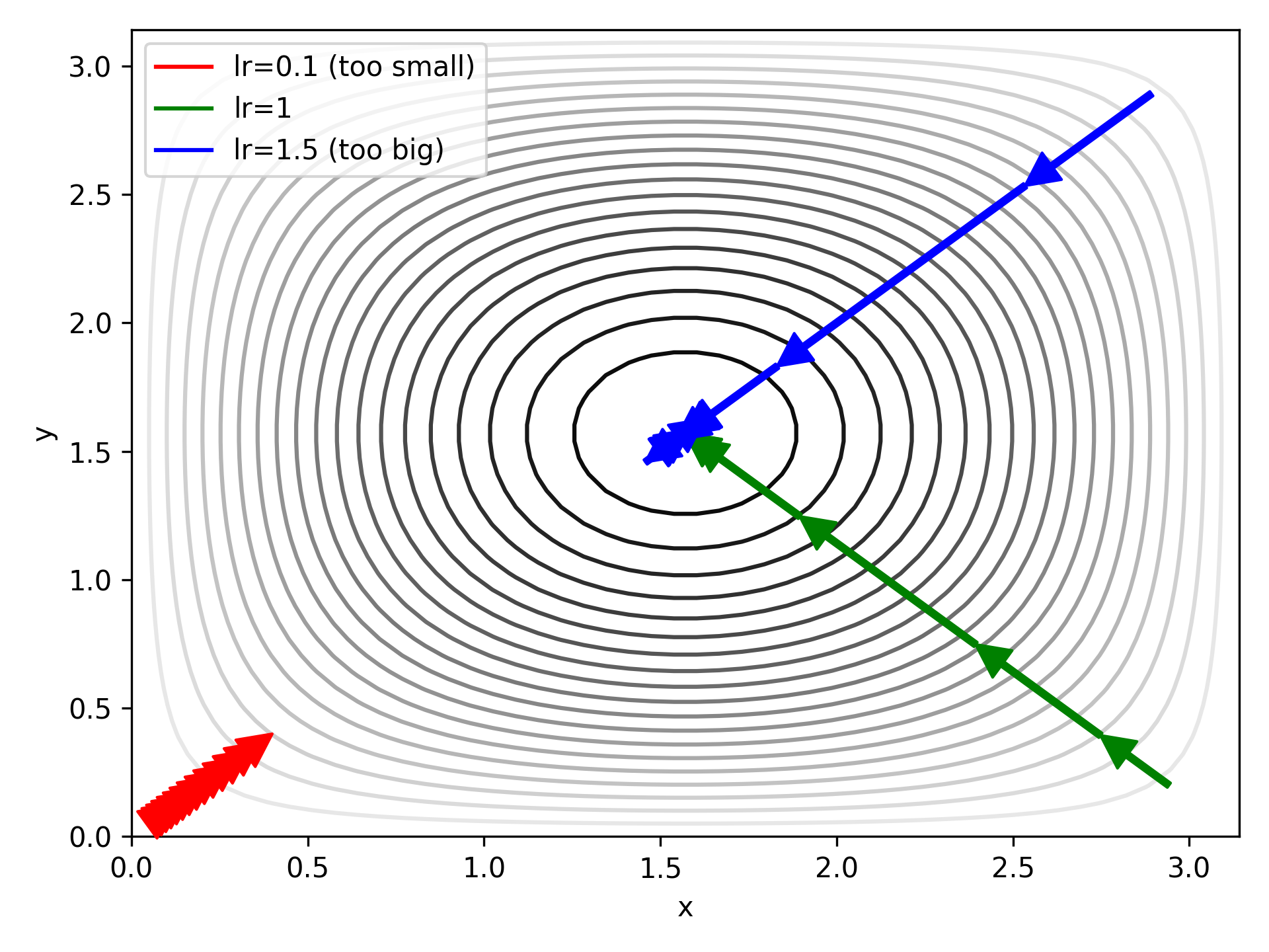
A large LR gets us closer to the target, faster, but not with accuracy (blue arrows). A small LR doesn’t get us close enough (red arrows). If we happen upon the perfect LR for our problem it works out ok (green arrows), but this requires tuning by hand and, perhaps, fore-knowledge of the appriximate solution.

Could we vary LR to start large and decrease as we get closer to our target?

Learning Rate Scheduling

PyTorch has us covered here, too. There are a bunch of different schema of learning rate scheduling. Perhaps the simplest is just linearly reducing the learning rate from its starting value. More complex schemes involve increasing and decreasing the learning rate according to a cycle, or stepping down the learning rate only when the output (objective function) stagnates.

Let’s adapt pytorch_fopt again to include this. Again, this is fairly simple to do. We just need to create the scheduler object and give it the optimiser it is to update the LR of. ​

def pytorch_fopt(f: callable, a: torch.Tensor,
                 nfev=100,
                 opt=torch.optim.Adam,
                 sched=None,
                 opt_kwargs: dict = None,
                 sched_kwargs: dict = None):
    if opt_kwargs is None:
        opt_kwargs = dict()
    if sched_kwargs is None:
        sched_kwargs = dict()
    a.requires_grad = True
    opt = opt([a], **opt_kwargs)
    if sched is not None:
        sched = sched(opt, **sched_kwargs)
    v = torch.inf
    for _ in range(nfev):
        opt.zero_grad()
        v = f(*a)
        v.backward()
        opt.step()
        if sched is not None:
            sched.step()
    return v.detach().item(), a

Running this new version with a larger learning rate shows why this is useful. First, the base case (no scheduler):

pytorch_fopt(f,
             torch.zeros(2)+0.1,
             nfev=1000,
             opt_kwargs=dict(lr=3),
             sched=None,
             sched_kwargs=None)
# result: -0.9870120286941528, tensor([1.4659, 1.4659])

With a large learning rate we still get pretty close, but significantly worse than before even with our large number of iterations.

Next, let’s add a scheduler - a simple linear reduction in LR:

pytorch_fopt(f,
             torch.zeros(2)+0.1,
             nfev=1000,
             opt_kwargs=dict(lr=3),
             sched=torch.optim.lr_scheduler.LinearLR,
             sched_kwargs=dict(
                 start_factor=0.25)))
# result: -0.9997626543045044, tensor([1.5567, 1.5567])

Oooh getting closer, much closer now. Let’s try a cosine annealing algorithm. This scheduler is meant for tricky systems with lots of minima. It starts by increasing the LR, then rapidly reducing the LR (faster than the linear scheduler). This is to (1) find the globa minimum (2) get a very accurate value for the minimum. Let’s see if it helps:

pytorch_fopt(f,
             torch.zeros(2)+0.1,
             nfev=1000,
             opt_kwargs=dict(lr=3),
             sched=torch.optim.lr_scheduler.CosineAnnealingLR,
             sched_kwargs=dict(
                 T_max=1000)))
# result: -1.0, tensor([1.5708, 1.5708])

Exact answer! (Exact as far as my display precision allows, anyway).

Benchmarking

Now that we have a decent general function optimiser developed, let’s see how it compares to other, traditional, optimisers available in scipy.

I am going to assess the methods in two categories: accuracy and speed. Accuracy being how close can the algorithm get to the correct answer, and speed how long it took to get there (in terms of number of function evaluations).

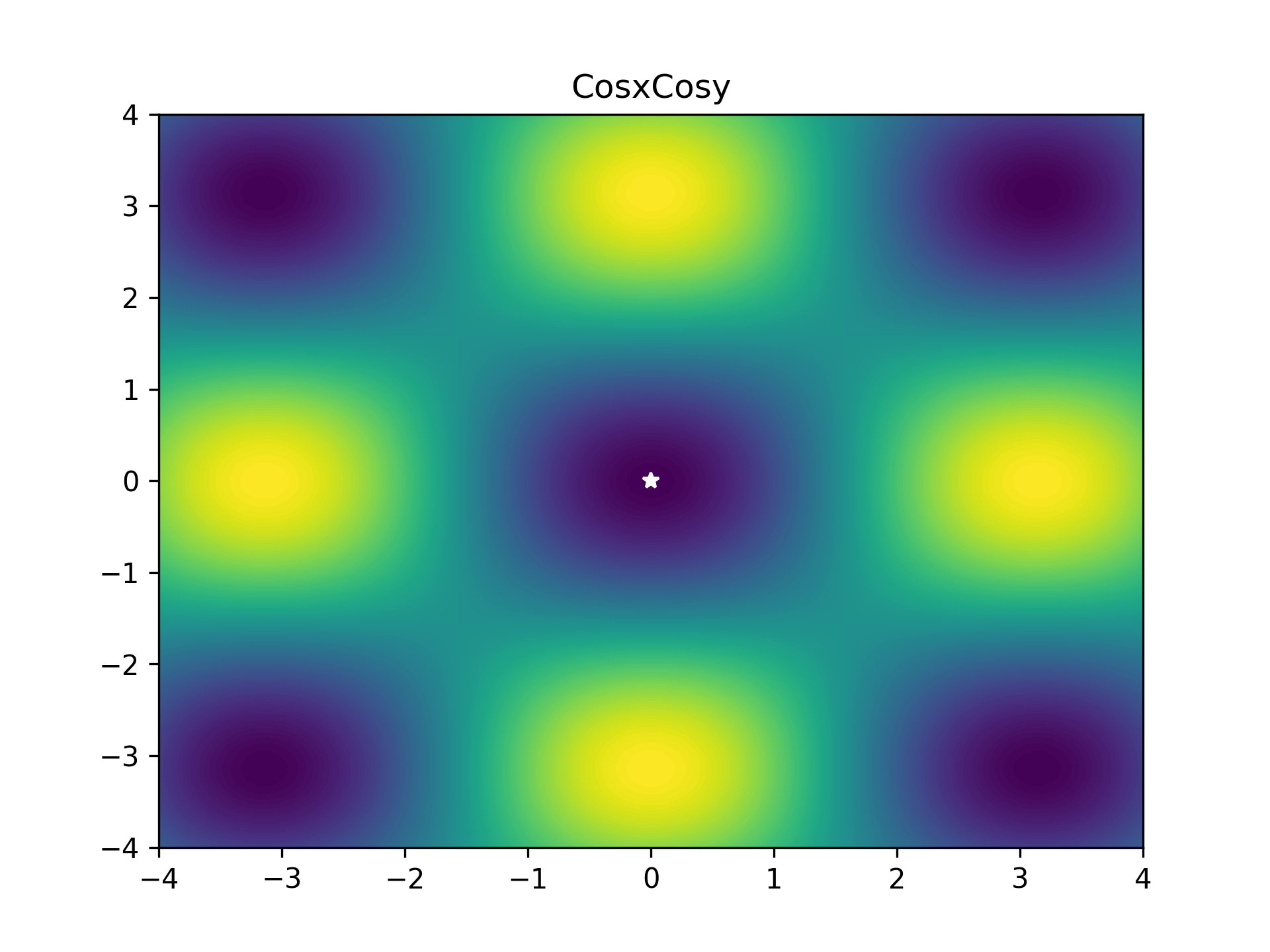
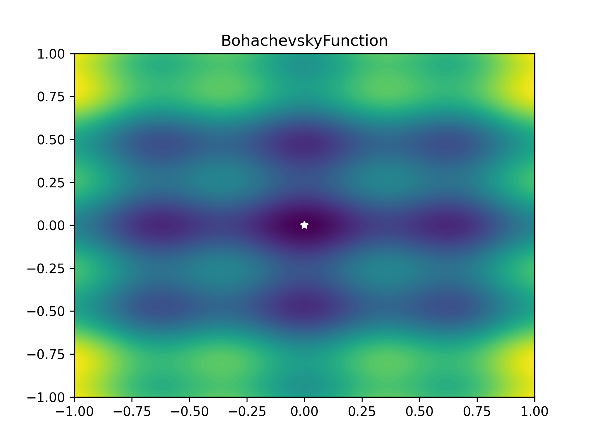
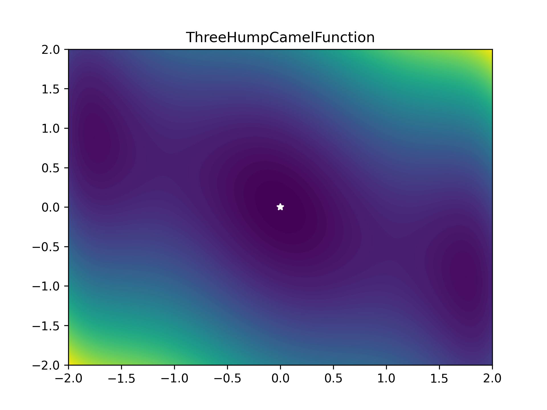
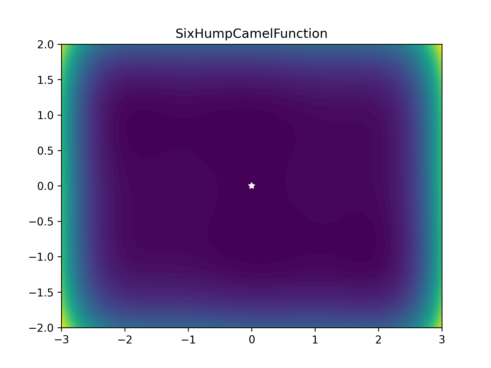
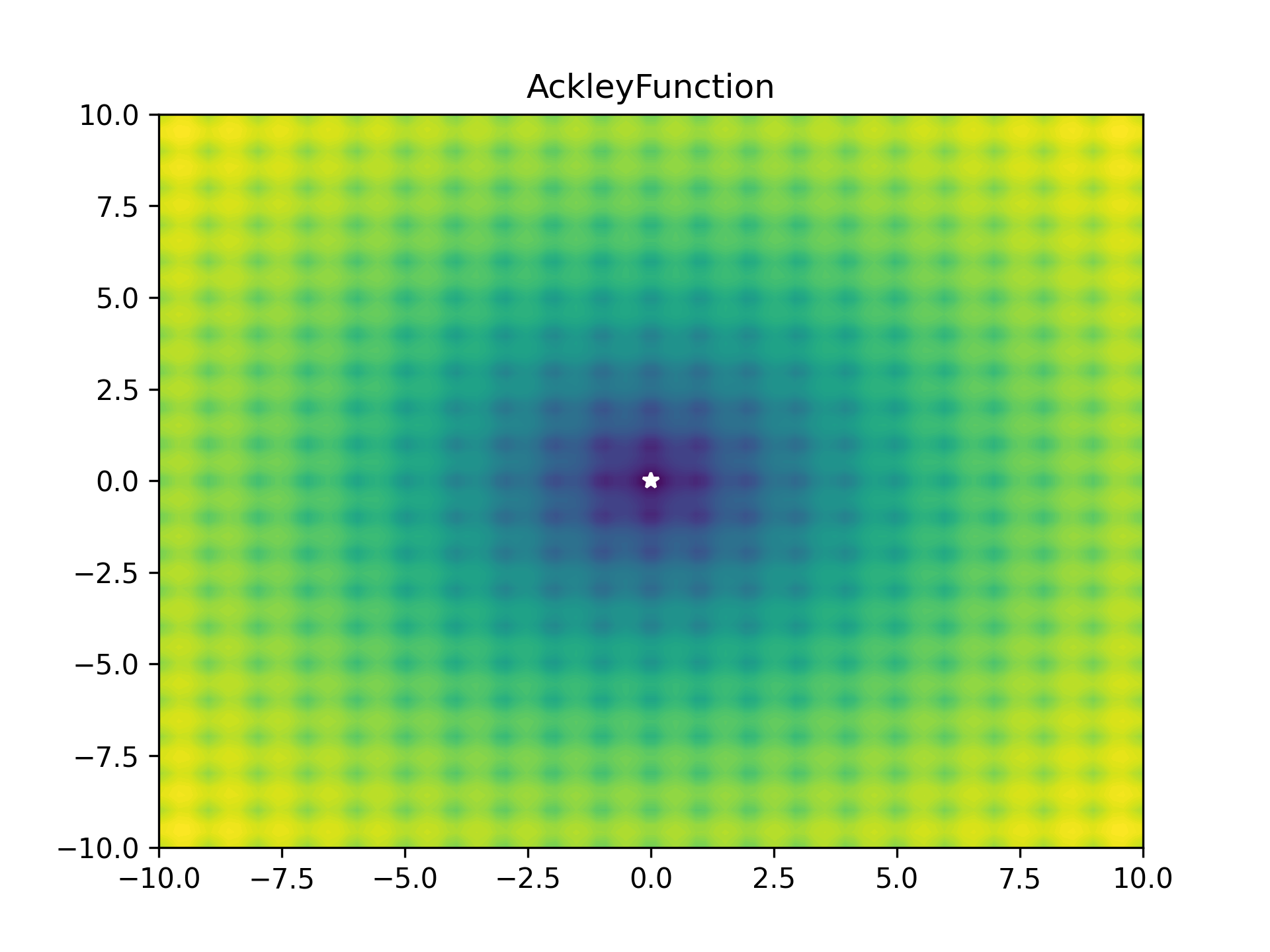
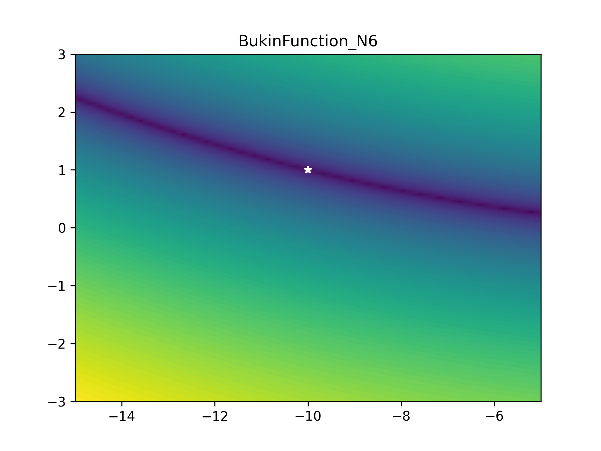
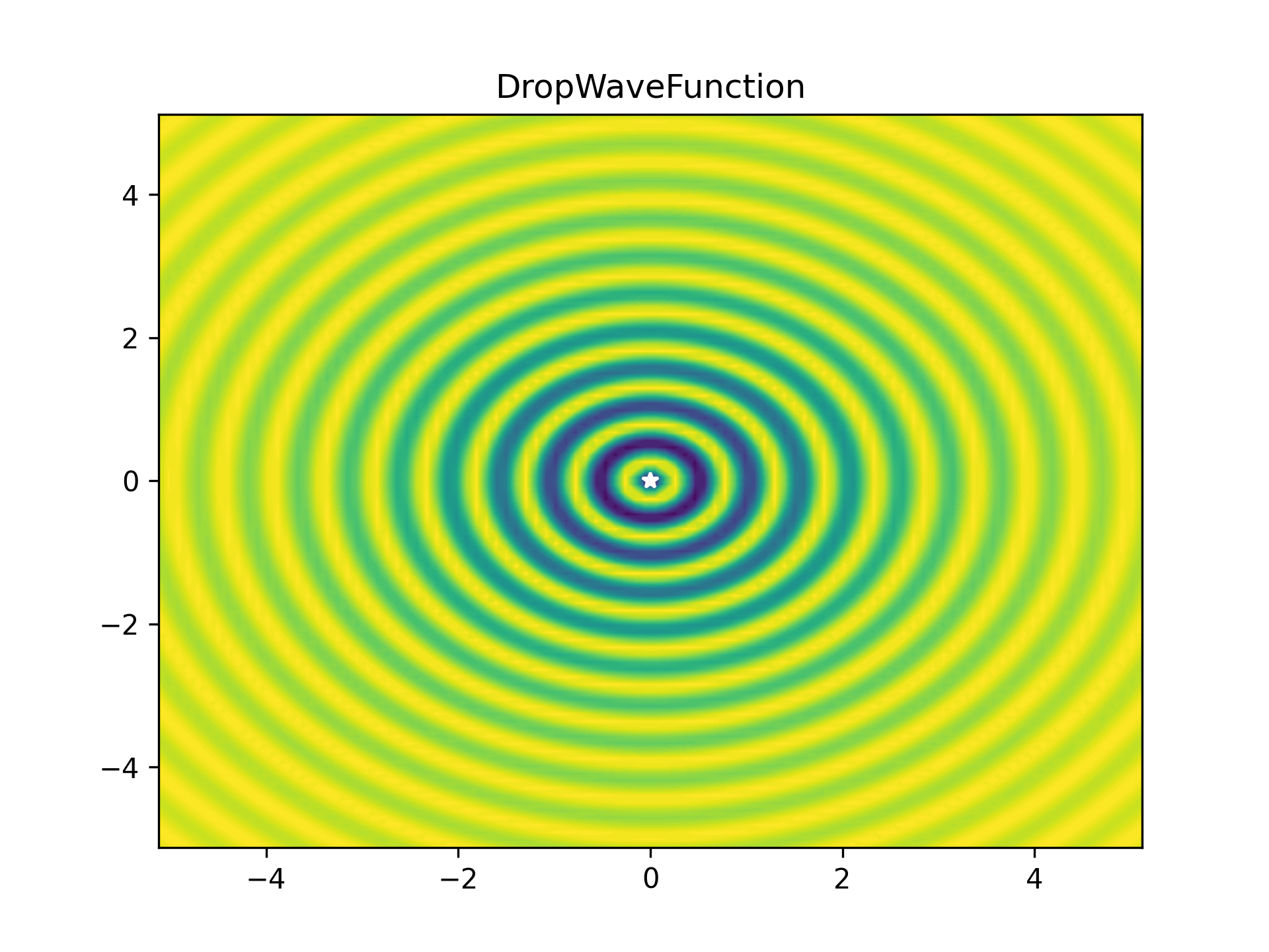
To benchmark the optimiser, I used a bunch of optimiser stress-test functions (most collected from here). These functions are plotted below as heatmaps. Large values are bright yellow, low values are dark blue/purple. They are in order approximately from easiest to hardest. The global minimum is represented as a white star. The functions have been modified so that this minimum lies on zero exactly.

As some competition for the PyTorch optimiser, some of Scipy’s optimisers were enlisted:

Scipy DualAnnealing

scipy.dual_annealing

Scipy BasinHopping

scipy.basinhopping

Scipy NelderMead

scipy.fmin

Two versions of the PyTorch optimiser were tested:

PyTorch Adam

Using Adam optimiser only and constant LR of 5% of the function bounds.

PyTorch SGD + StepLR

Stochastic Gradient Descent optimiser with a stepping LR decay scheduler (gamma of 0.8 and step size of 75)

Both PyTorch algorithms have a set maximum 10,000 number of function evaluations, and will stop early if the objective function falls below 0.001.

Running all the optimisers on all the functions gives us all the results, plotted below.

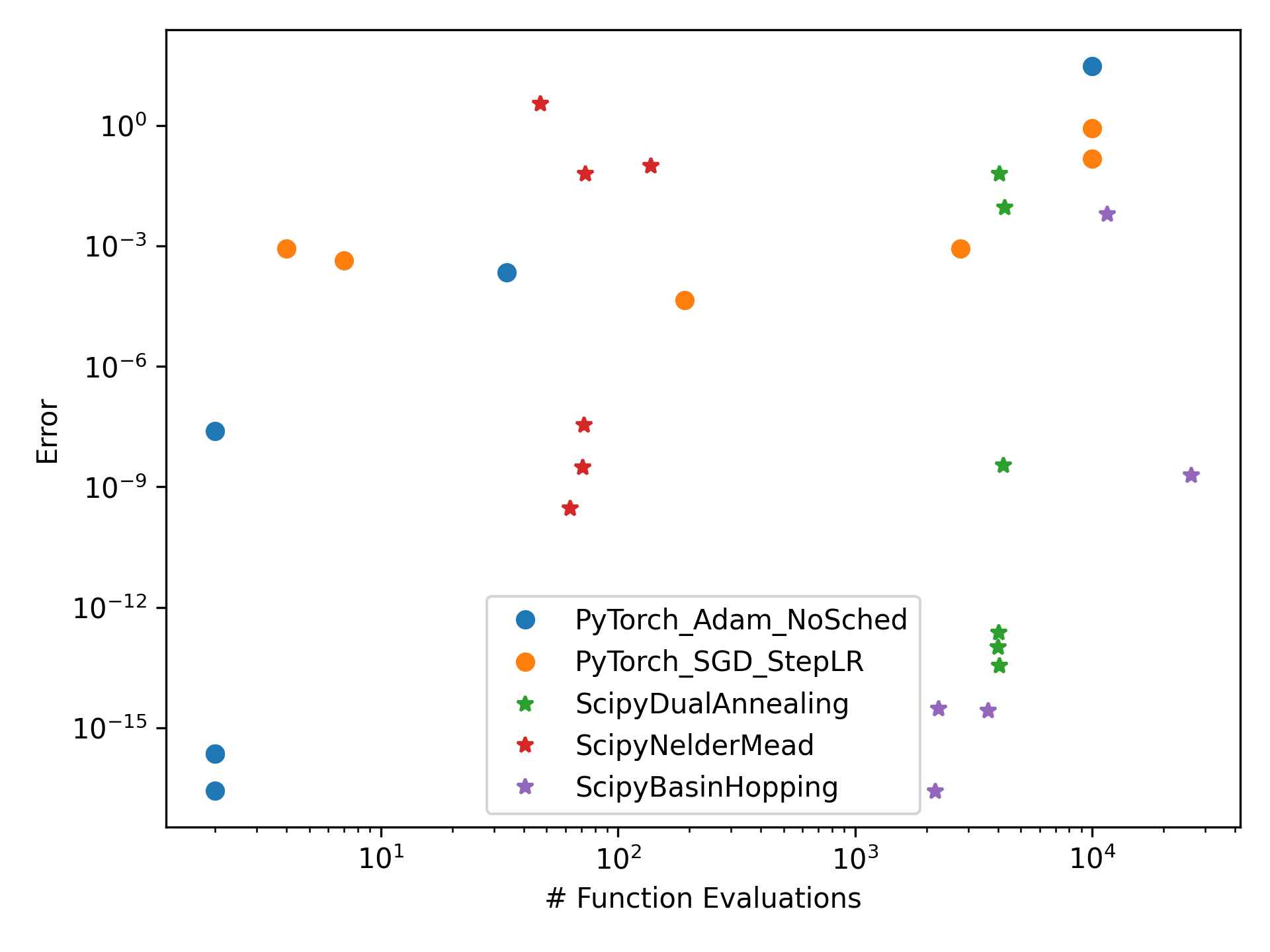
From the results we can see that PyTorch based optimisers vary wildly - being both the slowest (on the right hand side) and the fastest (some points on the left), also having the highest error (up top) and lowest error (bottom).

Scipy’s methods generally work really well but make consistently high number of function evaluations.

Conclusions

In this post I demonstrated how PyTorch can be (ab)used as a generic function optimiser useful for more than just machine learning. The autograd system is really very powerful and could be used for other cool stuff. If you have any ideas let me know in the comments below, or on twitter.

In comparing the PyTorch optimisers to scipy based ones we can see that pytorch_fopt can vary quite a lot - depending on how well tuned the optimiser is to the problem. Under favorable conditions, this can be extremely fast (< 10 evaluations) and with very low error (< 1e-15 ≈ 0). Scipy’s methods are much better generalists, performing with high accuracy most of the time, albeit always requiring 100+ evaluations.

In addition, a caveat should be noted for PyTorch based optimisers: the autograd system can be quite particular about the way functions are evaluated. In-line operations are not allowed, and all other maths must be done with torch methods. This is fine as torch is nearly a drop-in replacement for numpy, but should be kept in mind.